EventHPE: Event-based 3D Human Pose and Shape Estimation
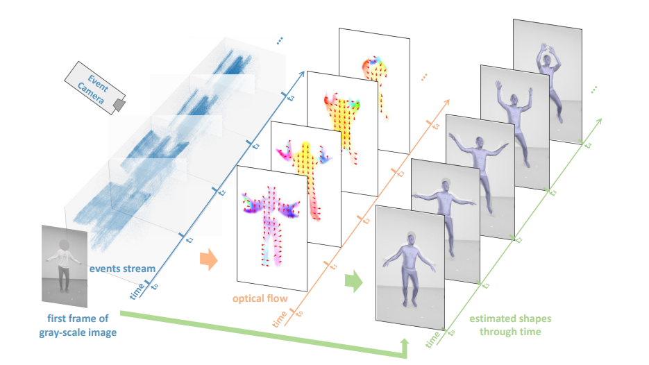
0. Abstract
- Two-stage deep learning approach
- FlowNet : Event 데이터 → unsupervised learning을 통해 optical flow 예측
- ShapeNet : Event & optical flow → 3D human shape 예측
- Novel flow coherence loss
1. Introduction
- 기존 : conventional RGB or RGB-D camera 기반
- Event camera 패러다임이 여러 분야에 적용되고 있으나, 3D HPE는 아직 미비함
- DHP19 [3] : Event packet → 2D pose 예측
- EventCap [28] : Event + gray-scale image sequence → 3D shape 예측
- Events는 시간에 따른 3D HPE를 수행하기 위한 유일한 입력 데이터로서, 첫 번째 프레임의 gray-scale에서 시작 형태가 알려져 있거나 추출된다는 가정하에 사용됨
- Contributions
- Event을 주로 사용해 3D human parametric shape 예측
- Gray-scale image sequence의 의존도를 낮추기 위해 optical flow 활용
- Coherence loss 도입
- Multi-Modality Human Pose and Shape Dataset (MMHPSD) 제작
- Event을 주로 사용해 3D human parametric shape 예측
2. Related Work
Human Pose and shape estimation
- Prior to deep learning : Primary dictionary learning-based
- SMPL [17]
- 인간의 body shape을 statistical low-dimensional하게 표현하는 방법
- End-to-end human shape estimation 가능
- HMR [13]
- SMPL 모델 활용, CNN 기반
- Single RGB image에서 human pose와 shape 예측 모델
Event camera and applications
- Event camera
- $(\mathbf x, t, p)$로 표현됨 ($\mathbf x$ : 픽셀 위치, $t$ : 발생 시간, $p$ : polarity)
- Preset threshold를 넘어갈 때만 발생 → asynchronous함
- Event camera Applications
- Camera pose estimation [8], feature tracking [10], optical flow [33], multi-view stereo [24], gesture recognition [1], motion deblurring [12]
3. Our Approach
Event camera
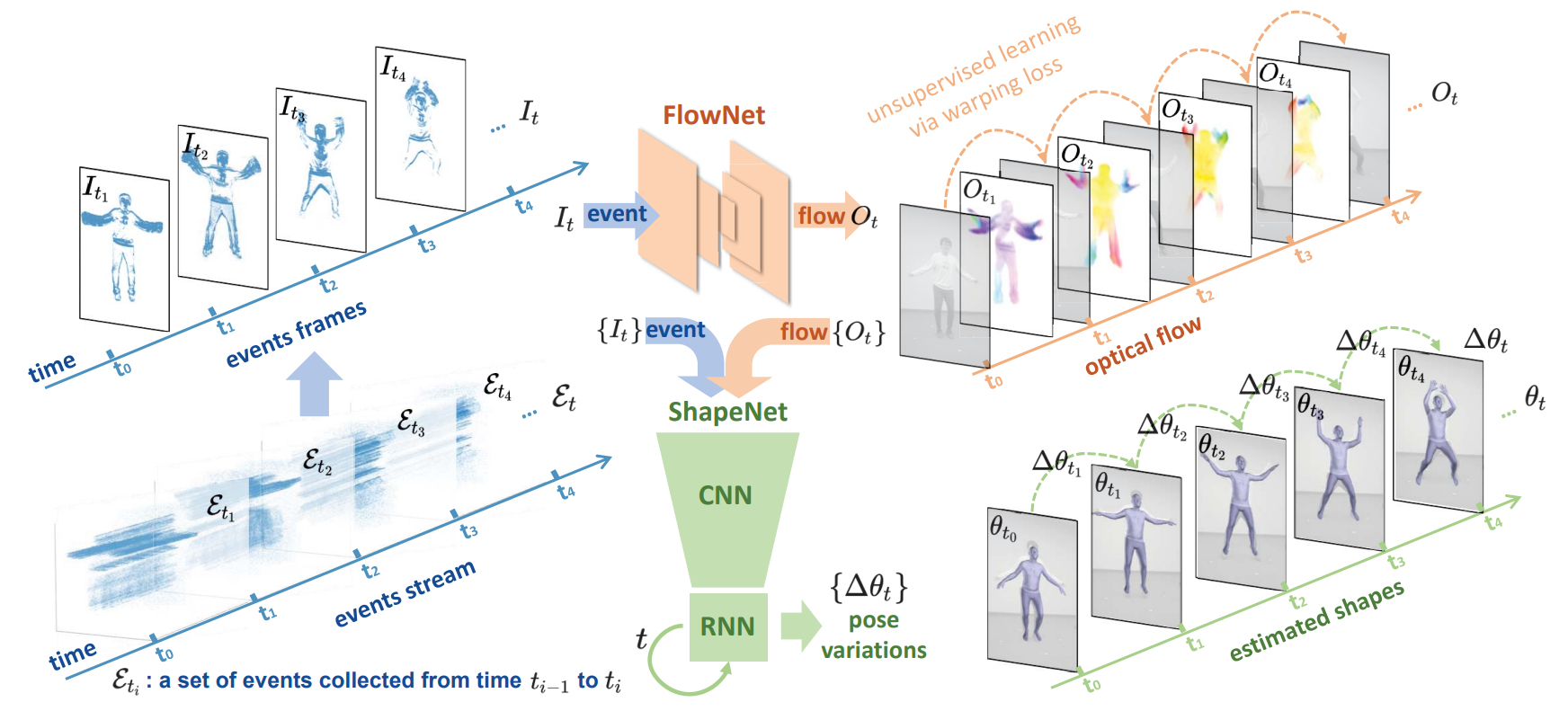
- Event stream은 N개의 event packet의 시퀀스로 분해됨 → $\mathcal E$
- \(\mathcal E = \{ \mathcal E_{t_i} \} _{i=1}^N\) , $\quad$ $\mathcal E_{t_i}$ : $t_{i-1}$에서 $t_i$사이의 event를 모은 것
- 각 패킷인 $\mathcal E_{t_i}$는 시간 순서에 의해 $M$개의 연속적인 subset으로 나누어짐
- 각각의 subset은 $I_{t_i}$라는 하나의 event frame 채널로 합쳐짐
M개의 연속적인 subset으로 나누는 이유는?
- 간단하지만 효과적으로 시간 정보를 포함할 수 있음
- Event camera 데이터를 정적으로 (static) 만들고, 파라미터를 눈에 보이게 변경
Human shape
- SMPL 모델로 표현
- 미분 가능한 함수, $\mathbf v = \mathcal M (\beta ,\theta ) \in \mathbb R^{6,890\times 3}$
- Output은 6890개의 정점(vertices)이 있는 triangular mesh
- Shape parameter $\beta \in \mathbb R^{10}$
- Body scan 데이터를 학습한 PCA shape space의 linear coeff.
- Body feature(키, 몸무게, 신체 비율 등)을 결정
- Pose paramaeter $\theta \in \mathbb R^{72}$
- 정확한 pose(global 혹은 relative rotation) 결정
- Shape parameter $\beta \in \mathbb R^{10}$
- Shape-dependent, pose-dependent 형태로 template body에 적용
- forward-kinematice로 template body shape를 target pose에 맞춤
- linear blend skinning으로 표면 mesh 변형
- 출력 mesh의 정점과 3D joint projection을 사용해 선형회귀 수행 → 2D, 3D 관절 위치($\mathbf J_{2D}, \mathbf J_{3D}$) 구할 수 있음
EventHPE
- Two-stage
- Event로부터 optical flow 예측
- Event stream → Event frame → CNN에 넣음
- 시간에 따른 shape 예측
- Event frame sequence와 해당하는 optical flow → CNN 통과 → vectorized feature representation 추출 → RNN 통과 → 매 시간 간격마다 pose variation, global translation variation 예측 - 첫 프레임의 pose와 shape은 알고 있거나, CNN 모델(e.g. VIBE [15])로 구해놓는다고 가정
- Event로부터 optical flow 예측
3.1 Unsupervised Learning of Optical Flow (FlowNet)
- 명확한 단서 추출을 위해 Event에서 optical flow를 추정
- Event frame $I_{t_i}$를 CNN 모델인 FlowNet에 입력 → optical flow $O_{t_i}$ 예측
- FlowNet : encoder-decoder 구조의 unsupervised 학습 모델
가져온 모델인가?
- Loss (EV-FlowNet [33]) : $\mathcal L_{optical-flow} = \mathcal L_{smooth} + \mathcal L_{photo}$
- 두 연속적인 gray-scale image ($I_{t_{i-1}}, I_{t_i}$) 사이의 loss
- $O_{t_i}$ : 예측된 optical flow
- $\hat I_{t_i} $ : bilinear sampling을 통해 $I_{t_i}$를 $I_{t_{i-1}}$로 이동시킨 값
- Photo-metric loss : target 이미지와($I_{t_{i-1}}$) 이동한 이미지의($\hat{I}_{t_i}$) pixel-intensity 차이
- $\mathcal L_{photo}(u, v; I_{t_{i-1}}, I_{t_i}, O_{t_i}) =\sum \limits_{x,y}\rho(I_{t_{i-1}}(x, y) − I_{t_i}(x + u(x, y), y + v(x, y)))$
- $\rho$ : Charbonnier loss function, $\rho (x) = \sqrt {x^2 + \epsilon^2}$
- $(u, v)$ : $O_{t_i}$의 2D direction
- $\mathcal L_{photo}(u, v; I_{t_{i-1}}, I_{t_i}, O_{t_i}) =\sum \limits_{x,y}\rho(I_{t_{i-1}}(x, y) − I_{t_i}(x + u(x, y), y + v(x, y)))$
- Smoothness loss : in-pixel flow와 이웃 pixel flow의 차이를 최소화
- $\mathcal L_{smooth}(u, v; O_{t_i}) = \sum\limits_{x,y} \sum\limits_{i,j \in \mathcal N(x,y)} \rho(u(x, y) − u(i, j)) + \rho(v(x, y) − v(i, j))$
- $\mathcal N (x,y)$ : pixel $(x,y)$의 이웃
- $\mathcal L_{smooth}(u, v; O_{t_i}) = \sum\limits_{x,y} \sum\limits_{i,j \in \mathcal N(x,y)} \rho(u(x, y) − u(i, j)) + \rho(v(x, y) − v(i, j))$
3.2 Pose and Shape Estimation (ShapeNet)
- $(t_{i-1}, t_i)$ 사이의 event frame $I_{t_i}$, optical flow $O_{t_i}$ → CNN model → vectorized feature representation → RNN model(GRU 활용) → output
- Output
- $\Delta\boldsymbol{\hat{\theta}}_{t_i} \in \mathbb R^{144}$ : inter-frame pose variations
- $\Delta\mathbf{\hat d}_{t_i} \in \mathbb{R}^3$ : global translation variations
- \(\mathcal L_{trans} = \sum\limits_{t_i} \|\mathbf d_{t_i} - \mathbf {\hat d}_{t_i} \|^2_2\) ( \(\mathbf d_{t_i}\) : target, $\mathbf{\hat d}_{t_i}$ : predicted)
- Relative rotation에 대한 pose로 3D axis-angle representation (SMPL) 대신 6D representation 사용
- $t_i$ 에서 $j$ 번째 relative rotation : \(\boldsymbol{\hat \theta }^{j}_{t_i} = \mathbf {R}^{-1}\big (\mathbf {R}(\Delta \boldsymbol {\hat \theta }^{j}_{t_i})\mathbf {R}(\boldsymbol {\hat \theta }^{j}_{t_{i-1}})\big )\)
- $\mathbf R(·)$ : 6D rotational representation → 3 by 3 rotation matrix 변환 function
- $t_i$ 에서 $j$ 번째 relative rotation : \(\boldsymbol{\hat \theta }^{j}_{t_i} = \mathbf {R}^{-1}\big (\mathbf {R}(\Delta \boldsymbol {\hat \theta }^{j}_{t_i})\mathbf {R}(\boldsymbol {\hat \theta }^{j}_{t_{i-1}})\big )\)
- \[\mathcal{L}_{pose} = \sum_{t_i}\sum_{j} \arccos^2\left( \frac{\text{Tr}\big( \mathbf{R}(\boldsymbol{\theta}^{j}_{t_i})^{\top} \mathbf{R}(\boldsymbol{\hat{\theta}}^{j}_{t_i})\big )-1}{2}\right)\]
- $SO(3)$에서의 geodesic distance를 사용
$SO(3)$ : 3차원 회전을 나타내는 특수 직교 그룹. 3차원 회전 공간을 나타내며, 회전에 대한 연산을 다루는데 사용됨.
- 2D 및 3D joint의 position error도 고려
- \[\mathcal {L}_{3D} = \sum\limits_{t_i} \sum\limits_{j} \|\mathbf {J}^j_{3D, t_i} - \mathbf {\hat J}^j_{3D, t_i}\|^2_2\quad,\quad \mathcal {L}_{2D} = \sum\limits_{t_i} \sum\limits_{j} \|\mathbf {J}^j_{2D, t_i} - \pi (\mathbf {\hat J}^j_{3D, t_i})\|^2_2\]
- $\mathbf {\hat J}^j_{3D, t_i}$ : joint $j$에서 3D position 예측값, $\pi(·)$ : projection function
- \[\mathcal {L}_{3D} = \sum\limits_{t_i} \sum\limits_{j} \|\mathbf {J}^j_{3D, t_i} - \mathbf {\hat J}^j_{3D, t_i}\|^2_2\quad,\quad \mathcal {L}_{2D} = \sum\limits_{t_i} \sum\limits_{j} \|\mathbf {J}^j_{2D, t_i} - \pi (\mathbf {\hat J}^j_{3D, t_i})\|^2_2\]
Coherence Loss ($\mathcal {L}_{\text {flow}}$)
- Image-based flow와 shape-based flow의 coherence loss
- 두 flow 모두 인간 움직임에 기반 → motion estimation 문제를 정규화 → 안정적으로 학습, 일반화 성능 향상
- Optical flow → Image-based flow ( $\mathbf {F}^{\text {img}}_{t_i}$ )
- \[\mathbf {F}^{img}_{t_i} = \mathrm{BilinearSample}(O_{t_i}, \pi (\mathbf {\hat v}_{t_{i-1}}))\]
- Human body shape의 vertices 움직임 → Shape-based flow ($\mathbf {F}^{\text {shape}}_{t_i}$ )
- 2개의 연속적인 human body shape을 image에 projection → 대응하는 vertices의 움직임 계산
- \[\mathbf {F}^{\text {shape}}_{t_i} = \pi (\mathbf {\hat v}_{t_i}) - \pi (\mathbf {\hat v}_{t_{i-1}}) \quad , \quad \mathbf {F}^{\text {shape}}_{t_i} \in \mathbb R^{6890\times 2}\]
- Optical flow → Image-based flow ( $\mathbf {F}^{\text {img}}_{t_i}$ )
- \[\mathcal {L}_{flow} = \sum\limits _{t_i}\sum\limits_{v} \frac {\langle \mathbf {F}^{\text {shape}}_{t_{i}, v}, \mathbf {F}^{\text {img}}_{t_{i}, v}\rangle }{\|\mathbf {F}^{\text {shape}}_{t_{i}, v}\|_2 \cdot \|\mathbf {F}^{\text {img}}_{t_{i}, v}\|_2}\]
- 최종 loss : \(\mathcal {L}=\lambda_{\text {trans}}\mathcal {L}_{\text {trans}}+ \lambda _{\text {pose}}\mathcal {L}_{\text {pose}}+\nonumber \lambda _{3D}\mathcal {L}_{3D}+ \lambda_{2D}\mathcal {L}_{2D}+ \lambda_{flow}\mathcal {L}_{flow}\)
- $\lambda$는 각각의 loss 가중치
3.3 Our MMHPSD Dataset
Data Acquisition
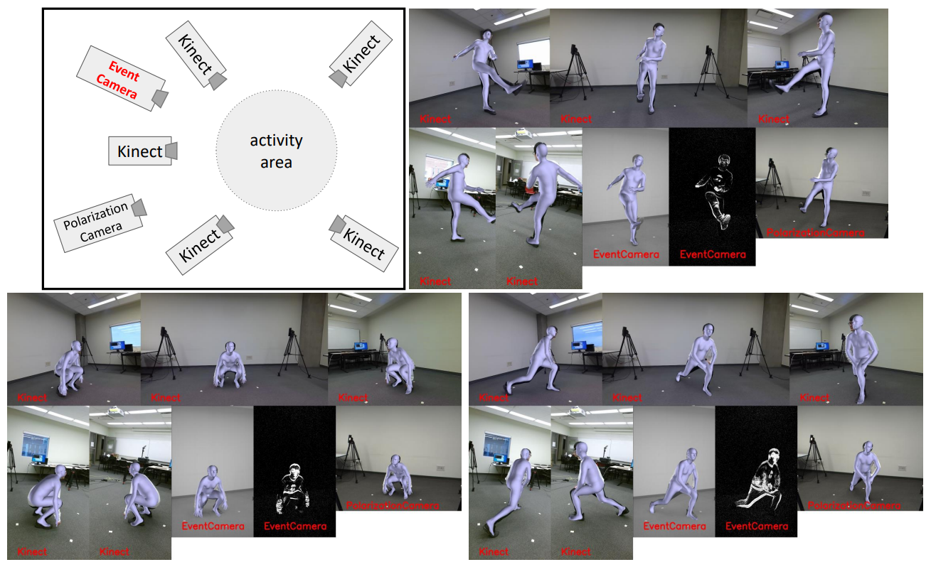
- Modality : event camera, polarization camera, RGB-D camera 등 4 종류의 modality 활용
- 두 gray-scale 이미지 사이의 event는 동기적으로 수집됨
- 15명의 참가자(11 남, 4 여)
- 각 참가자는 3개 그룹의 행동을 수행
- 빠른/중간/느린 속도로 진행되는 행동이 포함 → 총 21가지 다양한 행동이 수행됨
- 각 행동을 4회 반복
- 비디오는 대략 15 FPS, 약 1300프레임을 가짐
- 총 180개의 비디오 수집, 각 비디오의 지속 시간은 약 1.5분
- Dataset의 평균 이벤트 수는 초당 약 1백만
- 프레임 구성 : gray-scale image, 프레임 간 event sequence, polarity image, 5개의 RGB 및 depth image
Annotation
- 2D joint → OpenPose [4]
- 2D joint의 depth는 depth 이미지를 RGB 이미지에 맞추어 변형
- 5개의 카메라에서 얻는 초기 3D 자세 평균 → 남자 모델 피팅시켜 inital SMPL parameter 획득
- 5개의 depth view로 fine-tuning
- L-BFGS 알고리즘 사용 → shape vertices와 point cloud의 가장 가까운 지점의 평균 거리 최소화
Dataset Comparison
